| Issue 8 |
David started by giving us a large-scale example of the need for mass-flow measurement - the supply of fuel oil to a large container ship. The oil is sold by weight, but currently the measurement is often just of its volume - just a glorified dip-stick, of doubtful accuracy. The money involved is substantial, so there is clearly a need for something more precise.
|
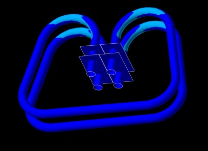
| Figure 1: Arrangement of mass-flow meter |
The Coriolis mass-flow meter measures fluid mass-flow (kg/s) by passing it through an arrangement of tubes which are undergoing angular vibration about an axis perpendicular to their length (Figure 1). The flow goes through both upper and lower tubes in the same direction, but their vibration is in opposite directions, driven by vertical "voice-coil" actuators acting up on one tube and down on the other at the left and right ends of the straight portions in the front of the picture.
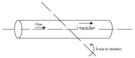
Consider flow along one of these straight tube lengths at the front of Figure 1 (see Figure 2).
|
| Figure 2: Flow along one of the straight tube lengths at the front of Figure 1 |
The Coriolis acceleration term is θ •r •θ, and is upwards for the directions shown (consider what happens to the vertical velocity of a fluid particle as it passes along the tube). The force to produce this acceleration of the fluid must come from somewhere, so there is a downward force on the tube. This force is proportional to the mass-flow rate, and is in phase with the sinusoidally varying angular velocity •θ. The tubes are thus set into a vertical vibration mode, superimposed on the angular mode. The design is such that the angular vibration is made to occur at the resonant frequency for that mode. The resonant frequency for vertical vibration is lower than for the angular mode (by a factor 1/√3 according to a simplified model, but slightly different in practice), so the vertical mode is excited somewhat above its resonant frequency by the Coriolis force. Its velocity therefore lags the driving force by 90°. Both frequencies will vary with the density of the fluid in the tubes, but the ratio between them should be constant. So if the vibration always occurs at the resonant frequency of the angular mode, the calibration factor should have a calculable relationship to this frequency, which of course can easily be measured.
The vertical velocity at each end of the tube is measured (electromagnetically). There will be a differential-mode component (one end up and one down) due to the angular vibration, and a common-mode component (up and down together) phase-shifted 90° from the other, due to the vertical vibration. The mass-flow rate can be shown to be proportional to the (small) phase difference between the combined velocities at each end.
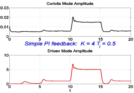
The main topic of the lecture was about how they (David and his research group) had devised a much-improved method of controlling the amplitude of angular vibration. The main disturbance to it occurs at the start of flow, when the tubes are only part full, and there is a lot of damping due to the sloshing of the fluid. To drive a resonant system at its resonant frequency, one needs a force in phase with velocity, which is equivalent to "negative damping". The initial approach was therefore to introduce a non-linear velocity-dependent force, with a positive term proportional to velocity and a negative term proportional to velocity cubed. This would give negative damping at small velocities, reducing and eventually changing sign as the amplitude increased. This does indeed control the amplitude, but not well enough, and introduces undesirable harmonics. So they tried an "amplitude-control loop", measuring the amplitude and varying the amount of negative damping with a simple proportional-plus-integral controller. Again, it works, but not well enough (Figure 3a). The shape of the step response varies with the amplitude of vibration, and there are undesirable overshoots and undershoots.
|
| Figure 3a: Amplitude-control loop behaviour |
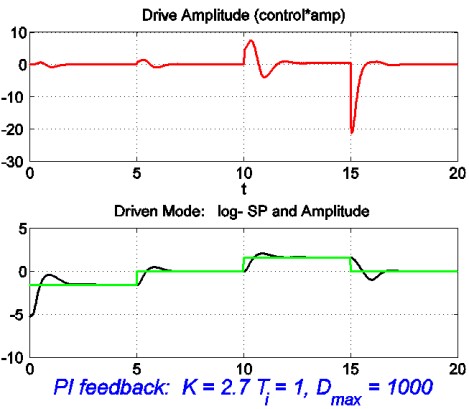
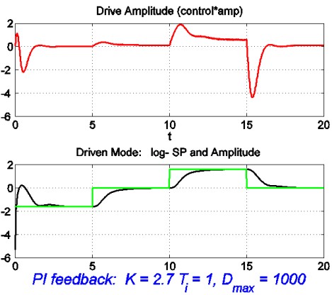
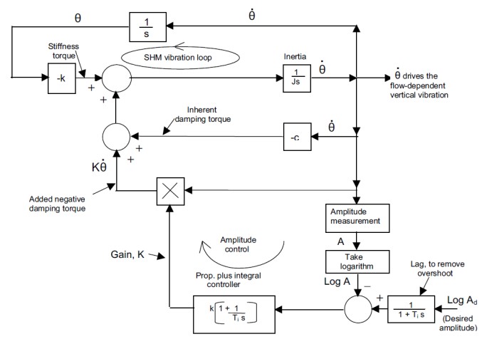
The cure for the amplitude-dependency of the step response is to base the gain-control loop on the logarithm of the amplitude, rather than on the amplitude itself. The overshoots and undershoots are then similar at all amplitudes, and are the natural result of a zero in the amplitude-control transfer function introduced by the proportional-plus-integral control algorithm (Figure 3b). The solution is simply to cancel the zero with an equivalent pole, by putting a simple lag transfer function immediately after the set-point input. The system is now as represented by the block diagram of Figure 4.
|
| Figure 3b: Log-amplitude control behaviour |
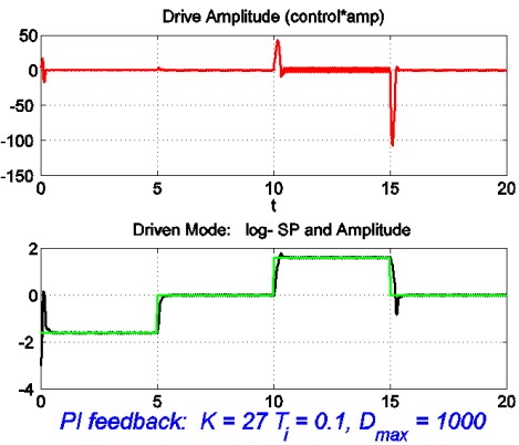
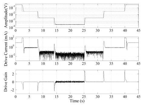
This was successful, but the response was at first a little slow (Figure 3c). Speeding it up by a factor of ten with suitable changes to gain and time constants brought overshoots back again at large amplitudes (Figure 3d). This was traced to saturation of the integral term (the finite range of a D-to-A converter). When this was cured the response was similar and well-behaved over three orders of magnitude of amplitude variation, as shown in Figure 5 for the actual system (the traces in Figure 3 are of simulations). At the smallest amplitude the current signal is noisy, but the amplitude is still behaving as it should. A comparison with a simple analog controller that had been used earlier showed substantial improvement.
|
| Figure 3c: Log-amplitude control behaviour with cancelled zero |
|
| Figure 3d: Log-amplitude control behaviour after speeding up |
|
| Figure 4: Block diagram of overall system |
|
| Figure 5: Behaviour of actual system |
For fire-safety reasons, when measuring the flow of fuel oil they are not allowed to put more than 25 mW of power into the drive coils. So if the damping increases significantly (air in the tubes), the amplitude must be decreased, but not allowed to vanish altogether, or the flow measurement will be lost. Hence the need for well-behaved control.
The complete algorithm, together with the other systems needed by the meter, were implemented by a combination of specialist circuit boards (DACs, ADCs, FPGAs etc.) and a host computer. A/D and D/A conversion was done to 24 bits, at a 48 kHz sampling rate. The amplitudes of the sinusoidal velocities were calculated, one cycle at a time, by a Fourier method, and the driving sinusoids were digitally synthesised. The design has led to a commercial product, mass-flow transmitter CFT50, built in the USA.
The work had won the Coriolis team the IET Measurement Prize for 2007. The team members are D Clarke, M Henry, M Tombs, F Zhou, M Duta, M Zamora, R Mercado, M Machacek, J Bowles and P Fair.
The lecture was supported by some impressive demonstrations, computer-driven displays from two projectors, and an actual vibrating tube set from a mass-flow meter, quite noisy if the amplitude of vibration was allowed to get too large.
| << Previous article | Contents | Next article >> |
| SOUE News Home |
Copyright © 2009 Society of Oxford University Engineers |
SOUE Home |